maph Tutorial

Introduction

maph is a command line tool for downstream network-based analysis of Proteomics and Phosphoproteomics data. The tool can be run on linux, Mac and Windows operating systems. What makes maph unique is it's ability to analyse your data at the phosphopeptide level thereby averting the need to manually map phosphopeptides to proteins.

Reactome annotates proteins in specific phosphorylation states as separate entities, therefore these phosphoproteins can take part in different signalling cascades depending on their phosphorylation state. Proteins in these differing modification states are hereby referred to as proteoforms. Taking advantage of this structure, maph takes an input file of phosphopeptides and maps the phosphorylations onto proteins and complexes according to a set of guidelines explained in detail in the figure below. It works by assigning a support score and an abundance score to each mapped protein and complex.

Support Score

Phosphoproteomic data is error prone therefore maph computes a support score to summarise the support we have in observing any given proteoform. maph does so by combining evidence from the data with that from knowledge bases such as Reactome into a support score for each proteoform. This support score summarises support for a given phosphorylation state of a protein (proteoform) over its other phosphorylation states based on observations from the data.

Proteoform - An entity in Reactome that represents the specific modified state of a protein. A protein could have two proteoforms representing its two phosphorylations states such as phosphorylation at a specific position and the unphosphorylated state.

To better understand how these scores are computed, it is important to first understand the structure of Reactome. The figure below outlines how Reactome is organised and shows its representation in maph.

Across all proteoforms (green), all recorded phosphorylations are aggregated into one group called Points of Interest (orange with each point being the vertical grey line) as shown in the figure below. The phosphorylations recorded in the Reactome network (in this example p^A, p^B, and p^C) are shown in purple while phosphorylations detected in the data (and not in the network) are shown in red.

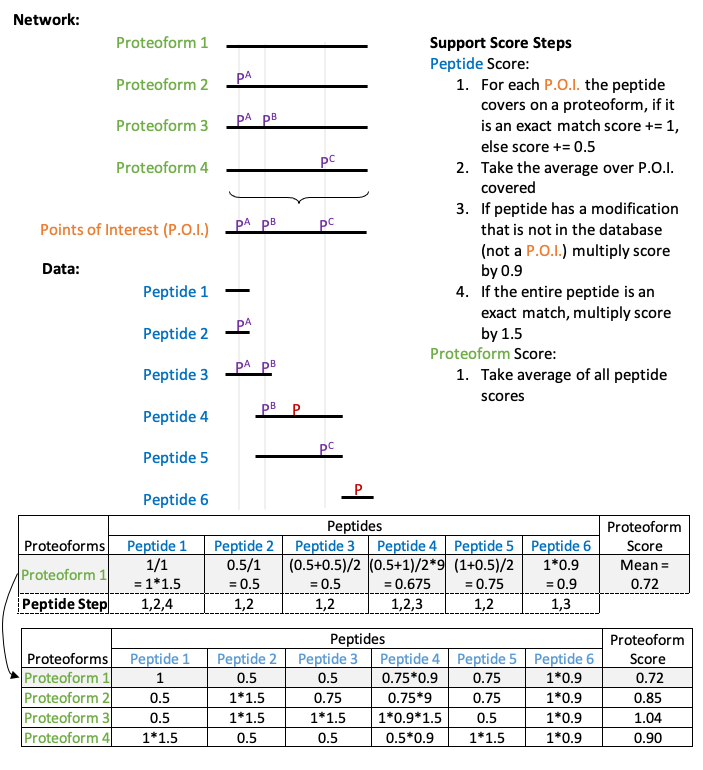
The rules in the figure above are used to determine the support we have in the presence of each proteoform given the data we have observed. The rules begin by evaluating the support each peptide brings towards a given proteoform. For instance, when evaluating support in proteoform 1, we look through peptides 1-6 and score the support they bring towards the existence of proteoform 1. Peptide 1 has no phosporylation marks at the corresponding point of interest in proteoform 1 therefore based on rule 1, it gets a score of 1. Since it overlaps only one point of interest, the averaged score across points of interest is 1 based on rule 2. Despite being a perfect match, it does not get up-weighted through rule 4 because it is unmodified.

Likewise, the score of peptide 4 towards proteoform 1 can be broken down as such:

1. The peptide overlaps two points of interest with the first being a match and the second being a mismatch thereby resulting in the scores 1 and 0.5 respectively based on rule 1.

2. Based on rule 2, the score over phosphorylations in the database are averaged therefore the score of this peptide is 0.75.

3. We observe a novel phosphorylation therefore based on rule 3, we down-weight the score by multiplying it by 0.9 thus resulting in the score of 0.675 for this peptide.

The scores contributions from all peptides are then aggregated using the mean to produce the final support score for each proteoform.

These rules have been logically derived to assist in the identification of high-support proteoforms. In rule 1 of the peptide score, a match means at the amino acid in the proteoform, and the peptide have the same status (both phosphorylated or both unphosphorylated). [We give a score of 0.5 for a mismatch because that peptide supports the existence of that proteoform, but we know that peptide contains a P.O.I. and will support another proteoform better]{.ul}. Next, looking at Rule 2, we take the average of all possible matches across points of interest to aggregate evidence from each individual point of interest. In Rule 3, we multiply the score by 0.9 to reflect that the database takes precedent over the data. However, we also reduce the weight of the score to reflect the extra unknown phosphorylation. Finally, in Rule 4, because a peptide mapping perfectly to a modified proteoform is uncommon and of interest we multiply the score by 1.5 to highlight the match.

Abundance Score

Concurrently but separately, abundances (e.g., intensity, SILAC ratio) or test statistics (e.g. log fold change) are mapped onto all proteins and complexes across the network. The process of computing this score is illustrated in the figure below. The default abundance score mapping takes the abundance from the peptide with the highest confidence score (if there are multiple peptides with the same confidence score the average of the abundances are taken). The user can also choose to compute the mean or median abundance for each phosphopeptide mapped to a proteoform.

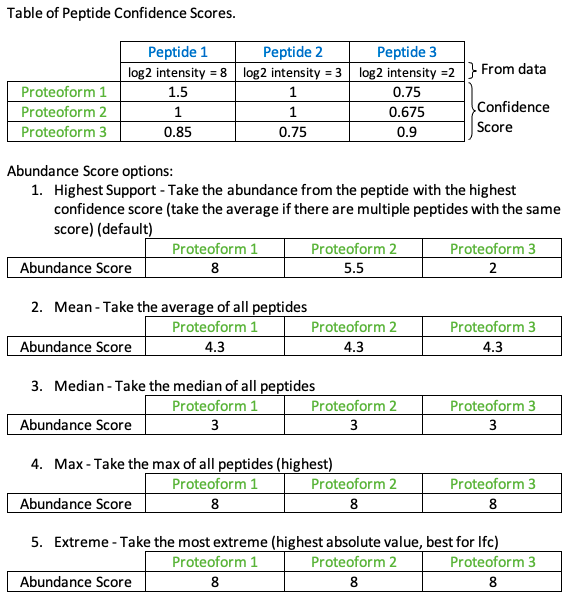
When the confidence score is mapped, the abundance score is mapped simultaneously, although the scores remain separate. The user has 4 options for mapping the abundance score as described above.

Combined, these scores provide a much better picture of the measurements allocated towards each proteoform. The workflow below demonstrates how these scores can be computed for a given data set and the additional benefit of interrogating the data using a network-based analytical framework.

Dependencies

• Java 8
• R
  • ggplot2
  • dplyr
  • viridis
  • ggExtra
  • devtools

If you do not have the required dependencies, the following conda command will create an environment called maph with all the dependencies installed.

conda create --name maph \
  --channel conda-forge \
  --channel bioconda \
  r=3.6 \
  r-devtools \
  r-ggplot2 \
  r-dplyr \
  r-viridis \
  r-ggExtra \
  openjdk=8

Setting up

**This is currently the Beta version. (Feb 4th 2022)

1. Clone this repo (as below) or create a new directory and place the provided scripts

git clone https://github.com/DavisLaboratory/maph.git

2. [OPTIONAL] download the most current version of Reactome and PhosphositePlus. There are currently pre-made integrated and non-integrated databases which can be found in the databases file in this repo for both human and mouse.

3. Map your data as shown in the section Mapping Phosphoproteomic Data.

4. Data can then be analysed with using various functions described below with detailed examples.

Analysis modes

maph is a suite of tools that enable a network-based analysis of phosphoproteomic data. The analysis tools provided within maph are in order of usage:

Database creation

1. CreateDB - This function is used to create the neo4j graph of Reactome.
2. IntegratePSP - This function with integrate the PhosphoSitePlus database into the Reactome graph created in the previous function.

Data mapping onto the database

1. MapPeptides - This function will map a phosphopeptide dataset onto the graph created in the previous steps. (can also be used for proteomics datasets)

Network analysis

1. TraversalAnalysis - This function performs the Traversal Analysis, which will generate a subgraph of everything up/downstream of the given UniProt IDs/nodes. A report will be generated along with a tsv file of the subgraph for cytoscape.
2. ShortestPath - This function will generate the shortest path between two given nodes, given such a path exists. A report is generated along with a tsv file for cytoscape.
3. MinimalConnectionNetwork - This function will create a subnetwork of all the shortest paths between all measured nodes of a given experiment. A report is generated along with a tsv file for cytoscape.
4. NeighbourhoodAnalysis - This function will highlight proteins and/or complexes that may not necessarily have been measured in the experiment itself but is surrounded by proteins and complexes that have been measured.
5. WriteDBtoSIF - This function will print the current graph as a SIF file (nodes and their edges) along with an attribute file (the properties belonging to each node. This function is intended to be used to allow the graph to be loaded and visualised in cytoscape.

Other accesory modules

1. ResetScores - This function will remove all scores for a given experiment label.
2. PrintDatabase - This function will print all nodes in the database onto the console.
3. AmountWithLabel - This function will tell you how many nodes in the graph there are with a given label. If no label is provided it will print out all current labels in the database.
4. WriteAllUIDs - This function will print all UniProt ids in the graph to the console.
5. WritePhos - This function will print all phosphorylations in the database to the console.
6. GetSpecies - This function will print the sprcies of a graph database.
7. PrintAllProperties - This function will print all properties in use of the given graph.
8. MapUIDs - This function will map a list of UniProt ids onto the database.
9. pSiteAnnotation - This fucntion will annotate phosphorylation sites on Gene Names.

Tool options and commands

To start, navigate into the repo directory and type the following command to view all of the tool options:

java -jar jars/maph.jar -h

The first 2 arguments are named -h (or --help) to access the above again (This will be useful later). While the second named option -m (or --mode) is used to specify which function you would like to perform. the current options are listed in the '{}' and then again below in a list form. As an example, the first option is:

"CreateDB", takes an OWL file [-iof], an output path [-op], an optional update boolean [-u] (can be T or F, default is T), and the species of graph you'd like to make [-s] (can be human (h) or mouse(m))

So if you would like to create a database you would put the CreateDB option after the -m when performing the command. However, this function requires a few parametes to be specified which are shown in the '[]'

For this option you will need to specify:

• the name of the input OWL file [-iof] of Reactome that you would like to build.
• the output directory where you'd like your graph to reside [-op]
• optionally you can specify if you'd like your database to be updated [-u] which can only be set to 'T' (true) or 'F' (false). (updating the database will update secondary UniProt accessions (reffered to here as UniProt ID's) to current UniProt ID's, it will also annotate any deleted or non-human UniProt ID's as deleted)
• you must also specify which species of database you'd like to create [-s], which can be set to Human with 'h', 'human', '9606', or Mouse 'm', 'mouse', '10090'

Thus, the final command would look something like this:

java -jar ./path/to/jars/maph.jar -m CreateDB -iof ./path/to/file/Reactome.owl -op ./path/to/graph/database/ -u T -s h

All comands will start with java -jar ./path/to/jars/maph.jar

Finally, below all the commands are all of the parameters required to run each command, and an explanation of that they are used for. e.g.,

• --input_owl_file [INPUT_OWL_FILE], -iof [INPUT_OWL_FILE] The OWL file to input

Mapping Phosphoproteomic Data

Now we should be ready to map our data! Data can be mapped to pre-built neo4j databases located in the databases folder, or you can build your own up-to-date database as shown above (see Creating a new integrated Database). The mapping process will modify the underlying graph database by computing and integrating confidence scores and abundance scores for each proteoform. To use the pre-computed databases in the databases directory, you will need to first extract the tar archives. You can do so using:

unzip databases/mouse.zip

Note that pre-computed databases need to be re-extracted for new analyses as the mapping step modifies the graph database.

In order to map your data you will need an input file with the following 4 columns;

1. A column where each cell contains a single UniProt ID corresponding to a peptide. The name of the column cannot contain spaces.
   • e.g., leading_razor_protein
2. A column specifying the modified peptide sequence. The name of the column cannot contain spaces.
   • The modified peptide may be one of 2 different formats. Either _(ac)AAAITDM(ox)ADLEELSRLS(ph)PLPPGS(ph)PGSAAR_ or AAAITDMADLEELSRLpSPLPPGpSPGSAAR
3. A column containing the value you would like mapped. The name of the column cannot contain spaces.
   • e.g., the column that holds: p-value, SILAC_ratio, log2_intensity
4. A column you would like the mapped values associated with, such as the experiment name or time. The name of the column cannot contain spaces.
   • e.g., the column that holds: stimulated, unstimulated, time_point_1

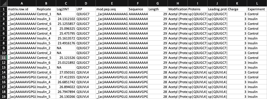
For demonstration purposes we will be mapping phosphoproteomic data generated by Humphrey et al., which can be found in ProteomeXchange underPXD001792. The dataset chosen for this tutorial is from the Mouse liver cell line FL38B where 6 replicates were treated with PBS (control) or Insulin. This data set was processed and select rows taken and made available in the exampleData directory of this git repository.

A quick look at the data:

For this example the parameters we set are:

1. LRP - The column containing uniprot IDs representing each peptide.
2. mod.pep.seq - The column representing the modified peptide sequence.
3. Log2INT - The column containing the statistic/value of interest that is to be mapped to each proteoform to obtain the abundance score.
4. Experiment - The column containing the experimental factor with which each statistic/value is associated.

With the data and the database ready, we can now proceed to mapping the data onto the database. The MapPeptides mode is used to perform this operation. This command is shown in the help guide as:

"MapPeptides", takes an input database [-idb] and an output path [-op], a file to map onto the database [-idf], and the optional Abundance Score mapping method preferred [-as] ("HighestSupport" is defalut)

Which needs the following parameters specified:

• the input database directory [-idb]
• the output directory for the mapping report [-op]
• the file of data you would like to map onto the database [-idf]
• The mapping option you'd prefer. There are 5 options 'HighestSupport', 'Max', 'Mean', 'Median', and 'Extreme'
  • Each option is explained above in the abundance score section. The default option is 'HighestSupport'.

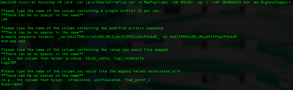
To map the data you can run the following command. Note that this is an intensive step and can take a few minutes to run depending on the size of your data. You will be prompted to enter the names of the four columns required to perform the mapping.

java -jar ./path/to/jars/maph.jar -m MapPeptides -idb ./path/to/graph/database/ -op ./path/to/output/ -idf ./path/to/data.txt -as HighestSupport

The tool will automatically detect the different experiments and map them separately. In this case, there are 2 experiments 'Control' and 'Insulin'. After mapping, we can look at the mapping report generated for each experiment in the output directory named 'PhosphoMappingReport_Control' and 'PhosphoMappingReport_Insulin' to understand how well each experiment mapped. Looking at the Control report:

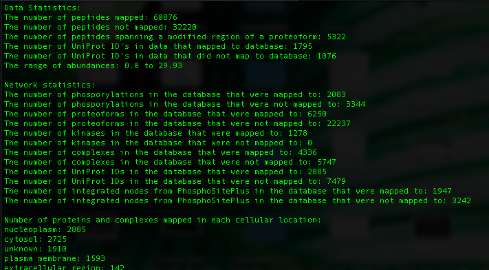
The first few lines give the statistics from the data such as the number of peptides and proteins that mapped and so on while the network statistics indicate the number of items in the database that were mapped to. Following that, the number of proteins and complexes that have been measured in each cellular location are shown in descending order.

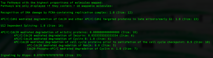
In addition, Reactome pathways with the highest proportion of measured proteins and complexes are listed. The proportion measured is shown at the end of each pathway along with the size of the pathway.

We can also look at our data in relation to qPhos. qPhos is a database holding 554 different experiments across 137 human cell lines. In order to provide context and to understand how well your experimental data mapped in relation to data from qPhos, we mapped all 554 experiments from qPhos to the integrated database and recorded numerous statistics. By running the provided Rscript command( Rscript -e "rmarkdown::render('proportionPlots.Rmd')" ) in the same directory as the provided 'R' directory you can visualize your experiment in relation to all qPhos experiments along with other general mapping information.

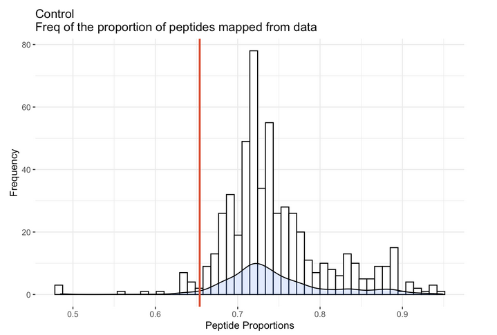
This plot from the R report depicts the distribution of the proportion of peptides mapped from each of the 554 qPhos experiments and where the Control experiment sits (the red line) in comparison.

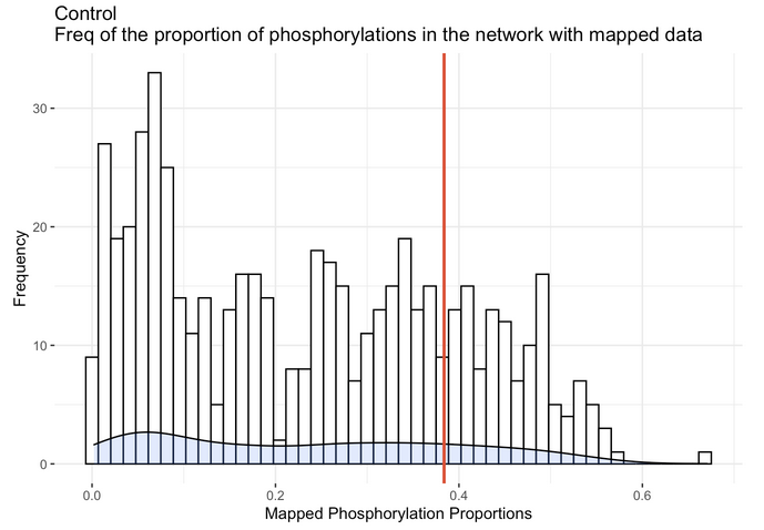
This plot depicts the distribution of the proportion of phosphorylation nodes in the database that were mapped to from each of the 554 qPhos experiments and where the Control experiment sits (the red line) in comparison.

Visualization

Cytoscape

After the data is mapped onto the database, you can write it to a Simple Interaction Format (SIF) file and an accompanying node attributes file to import into Cytoscape. The SIF file will be named SIF.sif and can be renamed but must retain the .sif extension. An example of a SIF file is:

21	INPUT	20
23	PHOSPHORYLATION	21
20	OUTPUT	24

Which we would read as the node with the id 21 is an INPUT to the reaction node with the id 20, or the node with the id 23 is a PHOSPHORYLATION on the node 21.

The attribute file will contain all attributes associated with each node. An example of an attribute file is:

Node_ID Database_ID Display_Name Type Database_Link Location Status Kinase Transcription_Factor Cell_Surface_Receptor UniProt_Gene_Name Integrated ABUNDANCE_SCORE_wt SUPPORT_SCORE_wt ABUNDANCE_SCORE_stim SUPPORT_SCORE_stim
21 Protein2090 p-S568-MLXIPL Protein http://www.reactome.org/cgi-bin/eventbrowser_st_id?ST_ID=R-HSA-163687.1 nucleoplasm   TRANSCRIPTION_FACTOR  MLXIPL  3.2 0.9 -1.5 0.5
24 SmallMolecule848 Pi SmallMolecule http://www.reactome.org/cgi-bin/eventbrowser_st_id?ST_ID=R-ALL-113550.4 nucleoplasm           
20 BiochemicalReaction1310 [Dephosphorylation of pChREBP (Ser 568) by PP2A] BiochemicalReaction http://www.reactome.org/cgi-bin/eventbrowser_st_id?ST_ID=R-HSA-164056.2
23 Protein2090_p-S_568 p-S_568 p_S 568

Where the attributes are associated with the node ids found in the SIF file. The first line contains all of the attributes that are found in that database.

Attribute name	Description
Node_ID	The unique node number used to link nodes to attributes in Cytoscape
Database_ID	The unique node ID given by Reactome
Display_Name	The name of the node
Type	The type of node
Database_Link	The link to the database that has more information on the node. Can link back to Reactome, PhosphoSitePlus or UniProt
Location	The cellular location of the node
Status	The status of UniProt nodes, can be nothing (if the database was not updated), 'Current', 'Updated', or 'Deleted?' - the question mark indicates further review is needed. The UniProt Id could be old and outdated or not consistent with the species in the database.
Kinase	If the node is a Kinase this column with have the values 'KINASE' otherwise it will be left blank. These are the lists of kinases for Human, and Mouse.
Transcription_Factor	If the node is a Transcription Factor this column with have the values 'TRANSCRIPTION_FACTOR' otherwise it will be left blank. These are the lists of Transcription factors for Human, and Mouse.
Cell_Surface_Receptor	If the node is a Cell Surface Receptor this column with have the values 'CELL_SURFACE_RECEPTOR' otherwise it will be left blank. These are the lists of Cell surface receptors for Human and Mouse.
UniProt_Gene_Name	The gene name associated with that UniProt ID from UniProt.
Integrated	If the node is from PhosphoSitePlus the value will be True.
ABUNDANCE_SCORE_*	The abundance score mapped from the data for a node. There may be multiple Abundance scores in a single database derived from multiple experiments. Each row labelled ABUNDANCE_SCORE_* will contain the experiment name in the suffix in place of the *.
SUPPORT_SCORE_*	The support score mapped from the data for a node. There may be multiple Support scores in a single database derived from multiple experiments. Each row labelled SUPPORT_SCORE_* will contain the experiment name in the suffix in place of the *.
NBHD_entity_measured_pval_*	The pvalue for the neighbourhood surrounding this node in the "Number of entities measured per neighbourhood" category.
NBHD_uids_measured_pval_*	The pvalue for the neighbourhood surrounding this node in the "Number of UniProt ids measured per neighbourhood" category.
NBHD_avg_pval_*	The pvalue for the neighbourhood surrounding this node in the "Average support score per neighbourhood" category.
NBHD_sum_pval_*	The pvalue for the neighbourhood surrounding this node in the "Sum of support scores per neighbourhood" category.

"WriteDBtoSIF" , takes an input database [-idb] and an output path [-op]

To write the SIF and attribute files, maph requires the input database directory and the output directory path. The command is as follows:

java -jar ./path/to/jars/maph.jar -m WriteDBtoSIF -idb ./path/to/graph/ -op ./path/to/output/

The SIF file can then be loaded into Cytoscape by clicking the network button from the tool bar (highlighted in red in the figure below).

Next, navigate to your SIF file and open it. I do not recommend creating a network view at this stage as the network is quite large and may crash Cytoscape (layout computation is an intensive task). Following this, click the attribute file button from the tool bar (highlighted in red in the figure below).

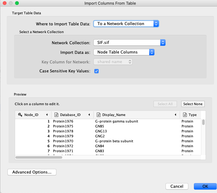
Navigate to your attribute file and open it. As in the figure below, make sure the Node_ID column is chosen as the key column. You can also change the value type of the attributes. One change you may like to make is to ensure the ABUNDANCE_SCORE_ and SUPPPORT_SCORE_ columns are set to numeric values.

Now your database should be ready to be explored. You may select multiple nodes from the node table and create a network view for the subnetwork induced by these nodes using the button highlighted in the figure below. Make sure to right click the highlighted nodes and choose 'Select nodes from selected rows' to ensure the nodes are selected.

Neo4j

To view and interact with the embedded neo4j database please follow these instructions:

1. Download and install the Neo4j (community edition), version 3.5.X as there is a compatibility issue with the later versions.
2. Untar/unzip Neo4j tar/zip file.
3. Copy your current mapped graph directory into a new directory named graph.db.
   1. You can do this in the command line using this command (for Mac/Linux): cp -r path/to/graph/ /graph.db/
4. Now that you have your graph.db directory, move it into /path/to/neo4j/data/databases/ and start it with the command:

• Mac/Linux: ./path/to/neo4j/bin/neo4j start (stop with ./path/to/neo4j/bin/neo4j stop).
• Windows: ./path/to/neo4j/bin/neo4j console (operations manual can be found here). Windows users will be prompted to enter authentication details (username: neo4j, password: neo4j) following which they will be prompted to change the password.

5. When the database is ready, you can open it to view in your localhost:7474
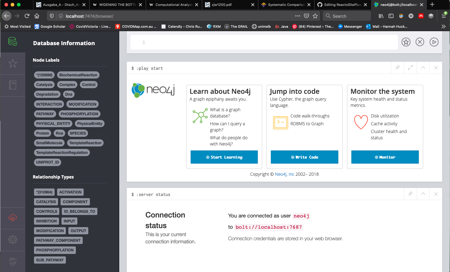
6. You can then use the Neo4j query language Cypher. An example of searching for a node by id is below (Query: MATCH (n) WHERE id(n) = 448 RETURN n).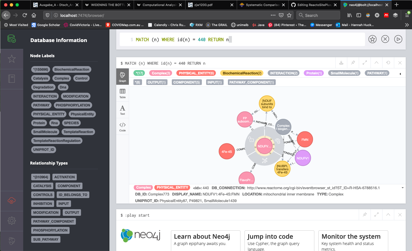

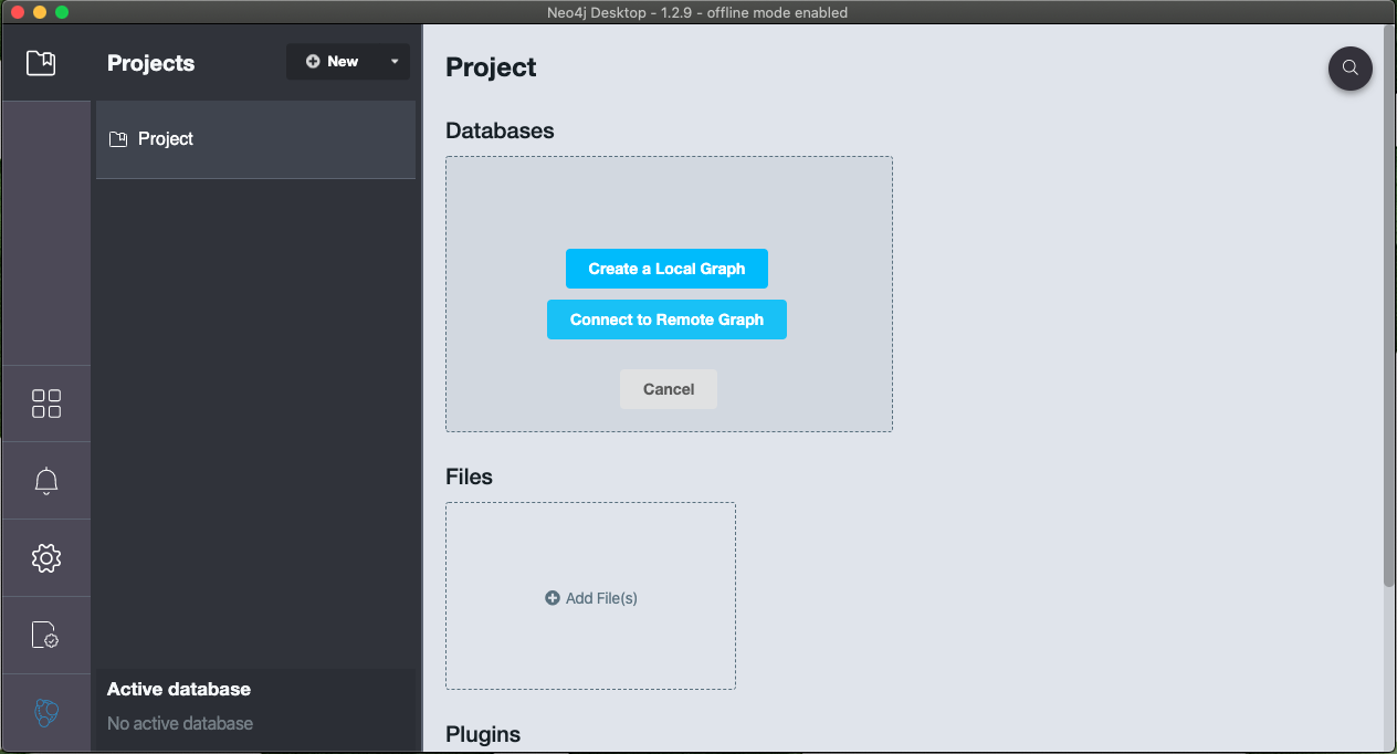
Alternatively, you can do this process manually in the Neo4j desktop app as shown below:

1. First open the app and make a new project
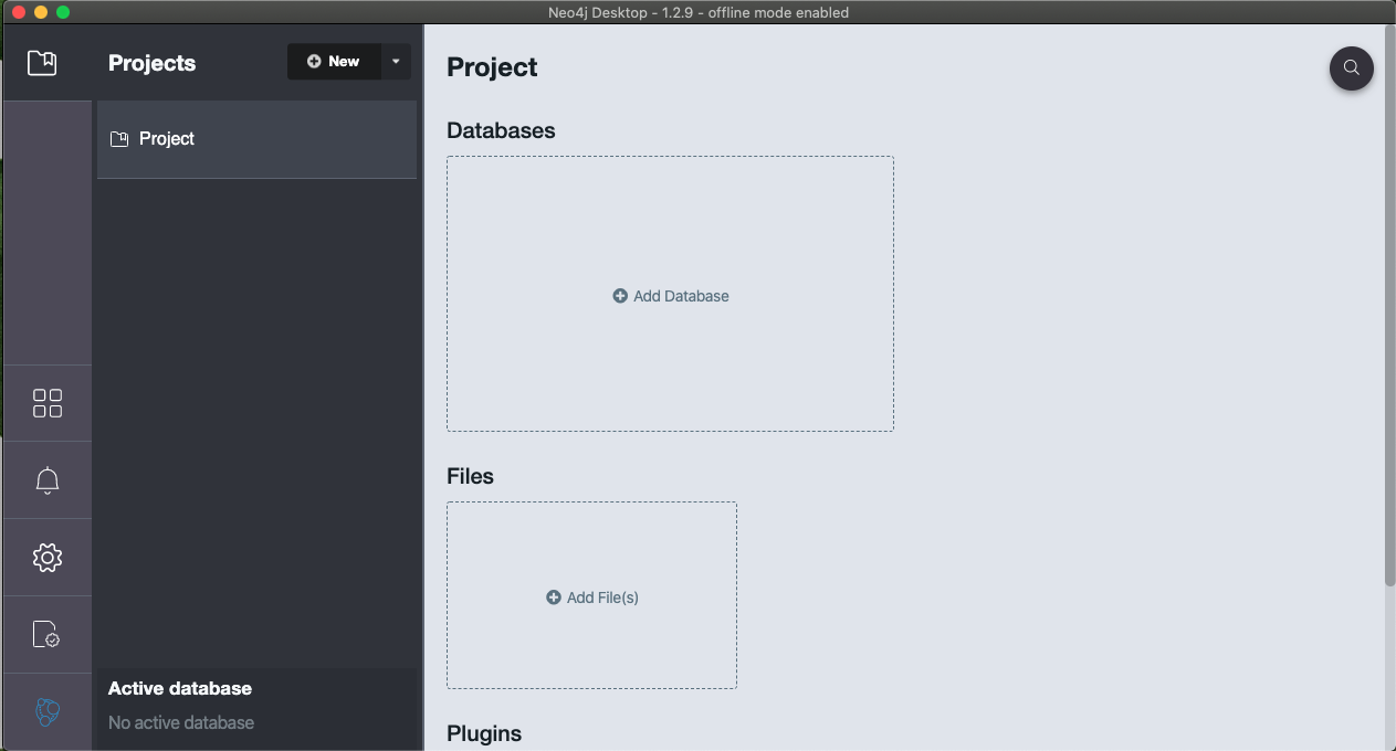
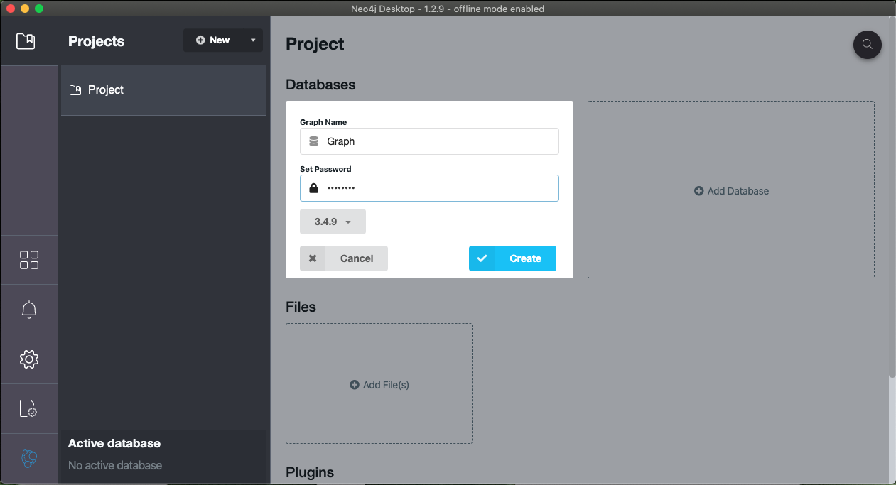
2. In the databases section, choose add database. Then, select 'create a local graph'
3. Set the name an password to your choosing and create
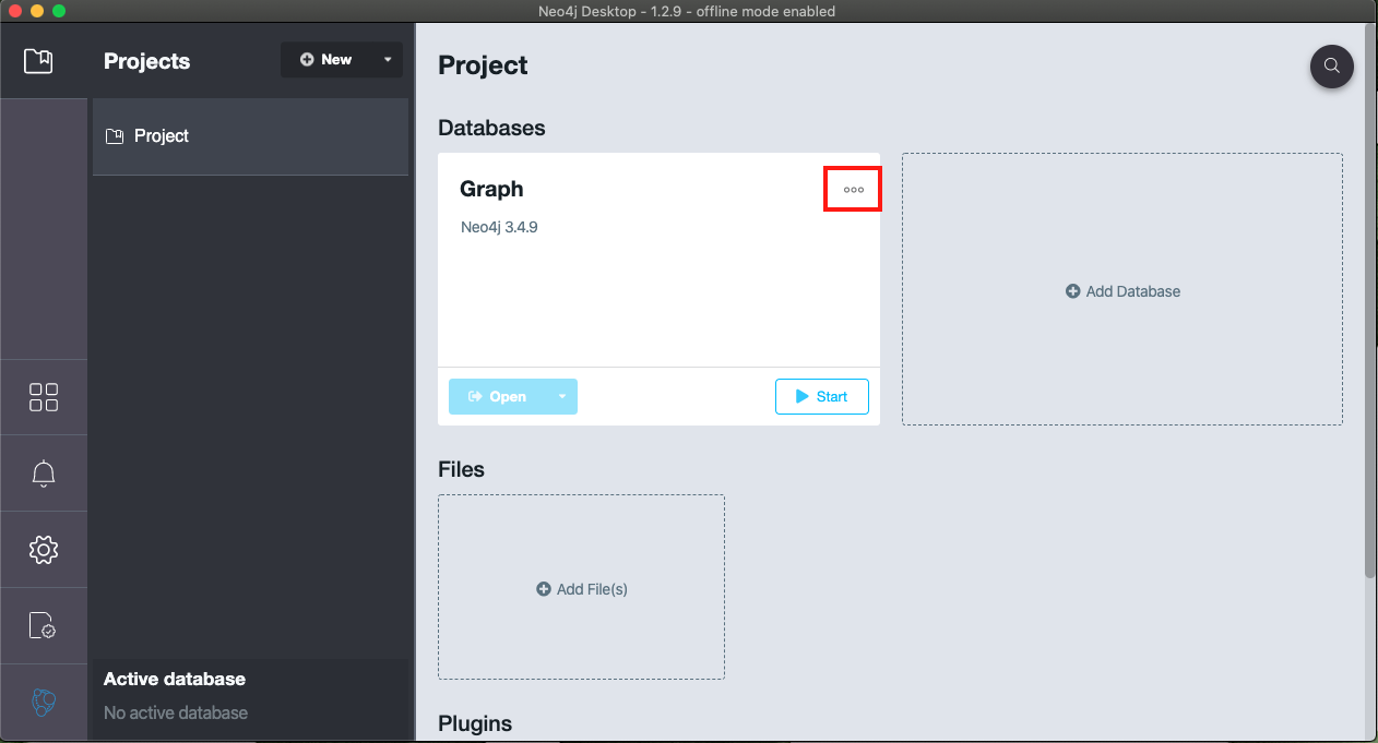
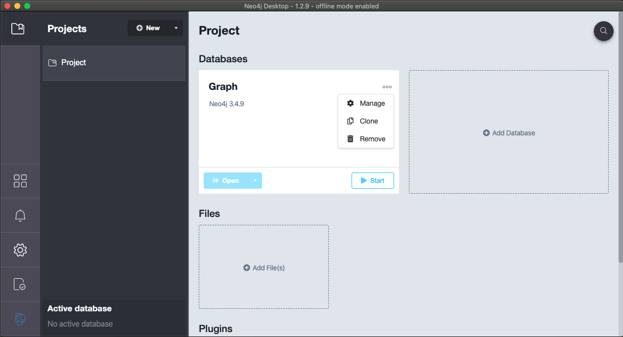
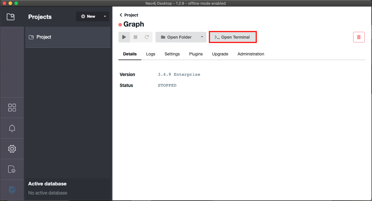
4. Then choose the menu in the top right-hand corner (highlighted in red) and select 'Manage database'
5. Next, select the open terminal button (highlighted in red)
6. Once the terminal is open you can copy your graph.db directory into the local directory. The command required is highlighted in red as well as available here (for Mac/Linux) : cp -r path/to/graph.db ./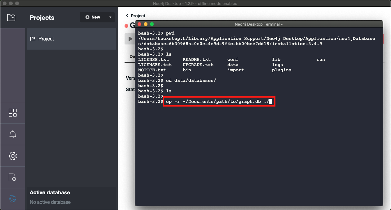
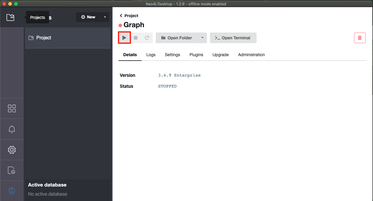
7. After the graph.db is in Neo4j, you can press play to start the local database. (highlighted in red)

More instructions are available from Neo4j and Reactome

Analysing Mapped Network

Now that the network has the data mapped to it, there are a number of ways to analyse the mapped network.

• Traversal analysis - Description
• Find the shortest path between two proteins - Description
• Neighbourhood analysis - Description
• Minimal Connection Network - Description
• Manual investigation via Cytoscape or Neo4j - Description

Traversal Analysis

With this function we can look at everything downstream or upstream of a protein of interest.

"TraversalAnalysis"", takes in a mapped input database [-idb], an output path [-op], a UniProt ID or database ID to look downstream of [-p], the direction of the traversal [-dir], and the experiment name of interest [-en].

Using the example data from earlier these are the function inputs for an analysis looking downstream of the mouse insulin receptor (Insr)(P15208):

java -jar jars/maph.jar -m TraversalAnalysis -idb ./path/to/graph/ -op ./path/to/output/ -p P15208 -dir downstream -en Control

We can look at the resulting report titled "TraversalReport_downstream_P15208.tsv":

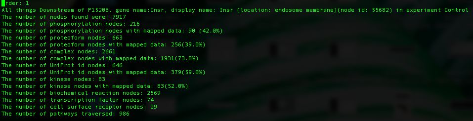
We see here that this UniProt ID has multiple proteoforms attached to it. Each may be in a different cellular location or have a different profile of modifications. The there a number of statistics reported for the downstream network of each proteoform and are ordered from largest to smallest (in reference to downstream network size). The first line is the variable names that can refer to that particular proteoform, next is the number of nodes found downstream of this proteoform. This statistic includes biochemical reaction nodes, gene nodes etc., as well as nodes that are mappable (proteins and complexes). The remaining statistics are self explanatory. This traversal will traverse all edges excepting small molecule edges, so as to avoid an explosion of things downstream of a single small molecule (for example ATP).

We can look at the downstream networks in Cytoscape by loading the file titled "P15208_downstream.tsv". Once this is loaded into Cytoscape and attached to our already loaded mapped network, we can filter the network to display the downstream networks of each proteoform.

Looking at the downstream network of Insr (node 55682) in Cytoscape we can start to investigate the differences in expression between experiments directly downstream of our protein of interest.

This function can also be performed on a particular node ID. This can be any node including "reaction" or "complex" nodes. An example of this function which retrieves the same network downstream of the insulin receptor is as follows :

java -jar jars/maph.jar -m TraversalAnalysis -idb ./path/to/graph/ -op ./path/to/output/ -p 55682 -dir downstream -en Control

Shortest Path

With this function you can look for the shortest path in the network between 2 proteins of interest.

"ShortestPath" takes in a mapped input database [-idb], an output path [-op], a starting node id [-sid], a ending node id [-eid], and the weight type to be traversed [-ew] (can be either "Abundance" (a) or "Support" (s)).

This algorithm will traverse all edge types with the exception of edges to and from small molecules. Using the example data from earlier we can look at the shortest path between the Insr (P15208) and the Jun protein node as seen in the traversal analysis earlier (node ID 20006):

java -jar jars/maph.jar -m ShortestPath -idb ./path/to/graph/ -op ./path/to/output/ -sid P15208 -eid 20006 -ew a

The function will never be able to find a path between 2 UniProt ID's (or UniProt ID nodes), only between UniProt ID's and node IDs, and node IDs to node IDs

We can look at the report titled "ShortestPath_P15208_to_20006.tsv":

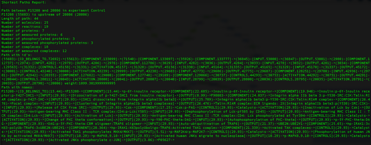
This function will report the shortest path between the 2 nodes in every experiment currently mapped on your database. The first line determines if the end node is up- or downstream of the starting node. Next a number of statistics are given. Finally, the path is shown with each node id and the total path weight, followed by the same path but with node names and the weight of each edge beside the reaction nodes.

We can visualize in Cytoscape by loading the file "P15208_to_20006_downstream.tsv ":

Neighbourhood Analysis

The neighbourhood analysis aims to highlight proteins and/or complexes that may not necessarily have been measured in the experiment itself but is surrounded by proteins and complexes that have been measured, making it a node of interest. To accomplish this, first an experiment must be mapped to the network, next a neighbourhood is generated around every protein and complex in the network. The number of direct neighbours to be traversed (and included in the neighbourhood) can be set by the user (henceforth referred to as the neighbourhood size), However, currently the only neighbourhood size available is 4. Certain edges are not traversed such as edges leaving small molecules (such as ATP (adenosine triphosphate), which is involved in hundreds of reactions) as well as component edges (which point to all the subcomponents of a complex) to avoid irrelevant reactions being included in the neighbourhood. Once a neighbourhood is generated, four measurements are taken. The first is the number of entities in the neighbourhood that have a received a mapping from the data, second is the number of UniProt ids in the neighbourhood that have received a mapping from the data. Third is the average support score (explained in detail in the manuscript) per neighbourhood and finally, the fourth measurement is the sum of support scores per neighbourhood.

Pre-calculated distributions have been calculated for each neighbourhood of varying experimental sizes against which you can compare your mapped data. As explained above, qPhos is a database holding 137 different phosphoproteomic experiments across 554 different human experimental conditions, while a database of mouse phosphoproteomics was developed in-house containing 33 experiments accross 680 different mouse experimental conditions [10.5281/zenodo.6370993].

Several empirical null distributions were pre-generated in order to calculate statistical significance of each neighbourhood in each of the four categories outined above. These distributions were generated for each species over a range of experiment sizes (1000 unique UniProt ids, 2000 unique UniProt ids, and 6000 unique UniProt ids), allowing the user to pick the distribution closest to their experiment size when performing the neighbourhood analysis. (You can see the number of unique UniProt ids that mapped from your data in the mapping report generated when data is initally mapped to guide you choice in distribution size)

This function cannot be used with new user-generated databases due to the pre-generated distributions being generated based on node ids unique to the provided databases (found in the /databases folder in this git page) If you would like instructions on how to generate an Empirical Null distribution specific for your database and dataset size please contact me (Hannah Huckstep) directly.

Using the example data from earlier these are the function inputs:

java -jar jars/maph.jar -m NeighbourhoodAnalysis -idb ./path/to/graph/ -op ./path/to/output/ -en Control -d 4 -cdf /path/to/CumulativeDensityFile/mouse1000/

"NeighbourhoodAnalysis" takes in a measured input database [-idb], an output path [-op], the depth of the traversal [-d], the experiment name of interest [-en], and the directory containing the pre-calculated Cumulative Density Function (of the Empirical Null Dirtibutions) per neighbourhood [-cdf]

The cdf directory is provided in this repo, however you will need to unzip the folder you'd like to use

Minimal Connection Network

With this function you can generate the network of all shortest paths between all nodes (typically referred to as the shortest-paths network).

"MinimalConnectionNetwork" takes in a mapped input database [-idb], an output path [-op], the experiment name of interest [-en], and the weight type to be traversed [-ew] (can be either "Abundance" (a) or "Support" (s)).

Computing shortest paths between all nodes can be intensive therefore this analysis may take a few minutes to complete. Continuing with the example data the function call would be:

java -jar jars/maph.jar -m MinimalConnectionNetwork -idb ./path/to/graph/ -op ./path/to/output/ -en Control -ew a

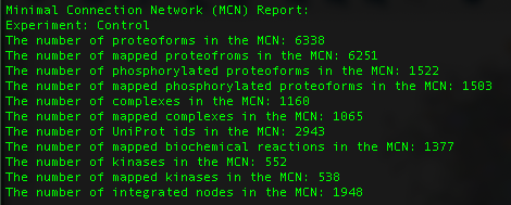
The report gives general statistics about what is found in the network by looking at "MinimalConnectionNetworkReport_Control.tsv".

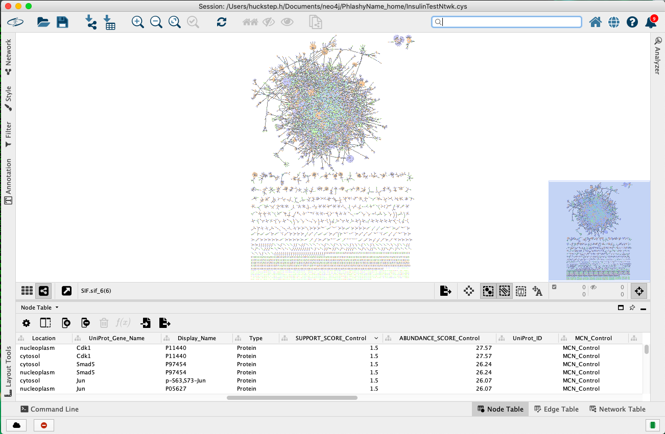
We can then visualize in Cytoscape by loading the file "MinimalConnectionNetworkReport_Control_Cytoscape.tsv"

Creating a new integrated Database

To create an embedded integrated database, first download the latest OWL files from Reactome and PhosphoSitePlus.

1. Download the latest Reactome database.
2. Untar/unzip Neo4j tar/zip file.
   • you can use either Homo_sapiens.owl or Mus_musculus.owl
3. Download the latest PhosphoSitePlus OWL file.
   • Navigate to the downloads section, choose 'Datasets from PSP'
   • Read and agree to terms and conditions
   • Download 'BioPAX:Kinase-substrate information'
4. Create the Reactome embedded database as shown above
   • e.g., java -jar ./path/to/jars/maph.jar -m CreateDB -iof ./path/to/file/Reactome.owl -op ./path/to/graph/ -u T -s h
   • Remember to specify wheather or not you'd like the database to be updated and the species
   • This function downloads many files live from UniProt. Therefore if internet access is unstable this function may crash. You can simply re-enter the command and it will overwrite the current failed output.
5. Once the Reactome graph is built, you can integrate with PhosphoSitePlus with the 'IntegratePSP' mode.
   • e.g., java -jar ./path/to/jars/maph.jar -m IntegratePSP -idb ./path/to/Reactome/Graph/ -op ./path/for/integration/report/output/ -iof ./path/to/PSP.owl
   • One key thing to remember is that the orgininal Reactome database that is input into this function is modified and becomes the integrated database.

Other Helpful Functions

AmountWithLabel

This function will print the number of things in the database with that label. For example:

"AmountWithLabel" takes in a input database [-idb], and a label type [-l].

java -jar ./path/to/jars/maph.jar -m AmountWithLabel -idb ./path/to/Reactome/Graph/ -l Protein

By inputting a non-existent label, this function will throw an error while showing all of the labels available for the given database.

PrintDatabase

This function will print every single node and edge with all of its properties to the console.

"PrintDatabase", takes in input database [-idb]

java -jar ./path/to/jars/maph.jar -m PrintDatabase -idb ./path/to/Reactome/Graph/

MapUIDs

This function will map a file containing a single UniProt id per line to the database (meant for lists of Proteins). It takes an input database [-idb], an output path[-op], an input data file [-idf], and a name to be assigned to the mapping [-mn]. This mapped data can then be used for any of the above functions. Please note, if performing a neighbourhood analysis with proteomics data the Average Support Score and Sum of Support Score categories will not be valid, if you'd like to use these categories please map data with the MapPeptides function (which will take non-phosphorylated peptides)

java -jar ./path/to/jars/maph.jar -m MapUIDs -idb ./path/to/Reactome/Graph/ -op ./path/to/output/ -idf ./path/to/data.txt -mn ProteinList

pSiteAnnotation

This function will take a MaxQuant Evidence file and will annotate the phosporylation sites found on each protein onto their respective gene name and add it on as a column to the end of the evidence file.

"pSiteAnnotation", takes an output path [-op] and an input data file [idf]"

e.g. will turn these "Q3UGC7", "_(ac)AAAAAAAAAAGDS(ph)DSWDADTFSMEDPVR_", "Eif3j1" into "Eif3j1_pS_14"

java -jar ./path/to/jars/maph.jar -m pSiteAnnotation -op ./path/to/output/ -idf ./path/to/data.txt

WriteAllUIDs

This function will write all UniProt ids in a given database into a file called “UniProtIDs.tsv”.

WritePhos

This function will write all Phosphorylations in a given database into a file called “Phosphorylations.tsv”. It will print the phosphorylations in the following format with the order UniProt id, modified amino acid, location. For example: Q9WTK7_p_Y166.

ResetScores

This function will remove all properties associated with a given experiment name. This includes “SUPPORT_SCORE”, “ABUNDANCE_SCORE”, “MAPPED”, “SCORED_BY”, “WEIGHT_SUPPORT” and “WEIGHT_ABUNDANCE”. if that experiment does not exist in the database, all current experiments in the database will be printed.

PrintAllProperties

This function will print all current node properties in a given database to the console.

---

Citations

Joshi-Tope G, Gillespie M, Vastrik I, D’Eustachio P, Schmidt E, de Bono B, et al. Reactome: A knowledgebase of biological pathways. Nucleic Acids Research. 2005;33(DATABASE ISS.). Jassal B, Matthews L, Viteri G, Gong C, Lorente P, Fabregat A, et al. The reactome pathway knowledgebase. Nucleic Acids Research. 2020 Jan 1;48(D1):D498–503. Hornbeck P v., Zhang B, Murray B, Kornhauser JM, Latham V, Skrzypek E. PhosphoSitePlus, 2014: mutations, PTMs and recalibrations. Nucleic Acids Research. 2015 Jan 28;43(D1):D512–20.